Spectrum Analyser
from KEUWLSOFT
Can be downloaded at Buy Me a Coffee (coffee optional).
Supporters on Patreon can find the app here.


Summary
Audio Spectrum Analyser for your Microphone. Feature include:
• 64 up to 8192 frequency divisions (128 to 16384 FFT size).
• 22 kHz spectrum range (can reduce down to 1 kHz for higher resolution).
• FFT windowing (Bartlett, Blackman, Flat Top, Hanning, Hamming, Tukey, Welch or none)
• Auto-scale or pinch to zoom, drag to pan.
• Linear or logarithmic scales.
• Peak frequency detection (polynomial fit).
• Averaging, Min and Max.
• Save CSV data files (uses Write External Storage Permission).
• Free or snap to peak cursor.
• Weighting - A, C or None. (A weighting filters the high and low frequencies according to how the ear perceives sound loudness).
• Octave Bands - Full, half, third, sixth, ninth or twelfth bands.
• Musical note indicator (green if within 5 cents, orange if within 10 cents).
• Auto-scaling microphone input trace.
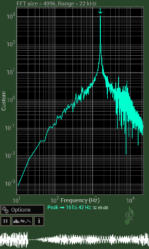
Screenshot 1 | 
Screenshot 2 |
FFT Size and FFT Range
The larger the FFT size, the greater the frequency resolution of the spectrum, but requiring longer processing times.
The FFT size can be set to 128, 256, 512, 1024, 2048, 4096, 8192 or 16384. Since a FFT spectrum contains real and imaginary components,
the extracted magnitude spectrum is only half the size. For best response on slower single core devices, keep the FFT size low.
The FFT range can be set to 1.1 kHz, 2.2 k Hz, 5.5 kHz, 11 kHz or 22 kHz. By performing an FFT over a smaller frequency range with
the same number of points, much better resolution can be achieved - although also requiring a longer sample of data.
FFT Window
A window can by applied to the time series data to reduce spectral leakage. Spectral leakage is more apparent at lower frequencies when
only a few waveforms fix into the data set. If an exact number of waveforms fit into the time series data set, there is no leakage, otherwise the amplitude of the peak
in the FFT will be reduced in amplitude and spread out. To reduce spectral leakage, the time series data can be multiplied by a window function which fades the
data to zero at both ends of the data set. The best window to use depends on the application. For example, Flat top would be used if you want good amplitude resolution, whilst a rectangular window (none) will give the
best frequency resolution.
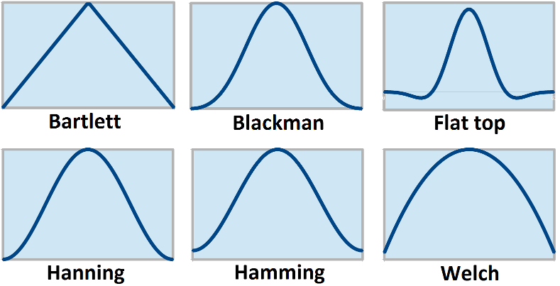
Bartlett, Blackman, Flat top, Hanning, Hamming and Welch windows
The Tukey window consists of a rectangular central section with cosine tapering at the edges. It has a parameter α that goes from 0 to 1 corresponding to the fraction of the window that is tapered. At α=0 it becomes a rectangular window and at α=1 it becomes a Hanning window. In the spectrum analyser app, α can be chosen to be 0.1, 0.2, 0.5 or 0.8.
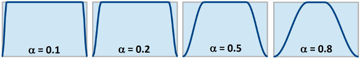
Tukey window
Weighting
Human hearing ranges from 20 Hz up to 20 kHz. The perceived loudness of sound varies over this range with sounds at the edges of this range perceived quieter.
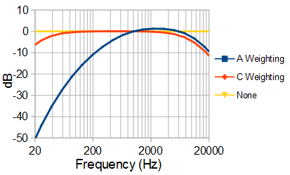
To take into account human hearing, the sound is often weighted based on its frequency to give a better indication of the sound level. The A and C weighting curves are defined in
IEC 61672:2003 with A weighing being the most commonly used. The following graph
shows how the three weighting options available in the app are applied over the 20-20kHz frequency range.
Octave Bands
The main trace can be shown as octave bands and toggled on or off by pressing the button between the pause and info buttons. This will toggle between trace, octave bands and combined modes. Each octave can be split into 1, 2, 3, 6, 9 or 12 bands as selected in the options menu. Bands are only shown when the frequency width of that band is at least 2 data points wide. Changing the FFT size and range will affect the number of bands shown. The centre frequency of the bands is based on 1kHz being the centre of one of the bands.
Axis Options
The X & Y axis can be set to automatically autoscale by selecting Options > Autoscale > ...
If not set to autoscale, or when paused, the trace can be made to fit the screen by
tapping the fit button. The graph can be zoomed or panned
by pinching or dragging the graph.
The X-axis shows frequency and can be set to be either a linear or logarithmic scale.
The Y-axis can show decibels, amplitude or intensity. The amplitude and intensity can
be shown on either linear or logarithmic scales.
The microphone input voltage is approximately proportional to sound pressure.
The power or intensity of sound is proportional to the sound pressure squared.
Decibels are a logarithmic way of representing the sound intensity relative to a reference value.
For this app, the reference is to the dB corresponding to saturating the microphone.
For the custom y-axis option, tapping setup will bring up another box in which the unit can be given a name and the full scale value entered.
The input unit is for the measured mic data in the time domain, The full scale value is the change in the new units in going from zero to full scale.
The FFT has the same y-axis unit but with the data plotted in the frequency domain.

Landscape screenshot
Averaging
Averaging can be turned on or off by selecting Options > Averaging When averaging the app will show the averaged trace in yellow. The peak of this averaged trace is also shown in the display below the graph. To reset the averaging, tap the zero button or go to Options > Averaging > Reset.
Max and Min
By selecting Options > Max & Min, traces for the maximum and minimum values recorded at each frequency can be shown. The maximum value from the maximum trace will be shown in the display below the graph. To reset the maximum and minimum traces, either tap the zero button, or go to Options > Max & Min > Reset
Interval
This option allows you to set the FFT update interval to 1 second, 500 ms, 250 ms or the fastest it can.
The actual FFT refresh rate will depend on the speed of the device.
When using a large FFTsize and/or low range, the length of data used can be greater than than the update interval
(up to 7.43 s for 16384 FFTsize and 1.1 kHz range).
Cursor
To turn the cursor on, go to Options > Cursor. The cursor can be set to be free or snap to peak. In snap to peak mode, the cursor will snap to any nearby peaks and the frequency & amplitude of that peak shown below the graph. In the free mode, the cursor will stay at the frequency you put it. To move the cursor, simply drag it to the desired location.
Saving Data
The spectrum data can be saved as a Comma Separated Values (CSV) data file.
Files are saved in the root directory with sequential numbering.
The first column is the frequency (in Hz). The remaining columns are for the current trace, and then if
used, the averaged, maximum and minimum traces. The values are in whatever y-axis
unit choice is currently selected. Below the FFT data, the raw time-series data for the current FFT is included, with columns of
time (s), Raw data (signed 16bit integer) & if windowing, the data after applying the window function.
Below the time series data is the values for each of the octave bands
Example data file:
Spectrum Analyzer Data File
2014-09-12 00:12:26
Frequency (Hz), dB,Average dB,Max dB,Min dB
0.0,-23.920067,-23.843828,-20.213928,-30.78797
34.453125,-31.675877,-31.634691,-20.734623,-70.90754
...
Time (s), Raw data,Windowed Data
0.0,-16.0,-0.0
2.2675737E-4,-15.0,-0.4761902
...
Twelfth Octave Bands
Center Frequency (Hz), dB
2996.6143,-58.675697
3174.8020,-55.430584
...
Store / Recall Setup
Within the Save menu, there is the option to save or recall the current setup to one of 5 memory slots. Scaling, averaging, FFT size, FFT window, ... settings are stored/retrieved.
On recalling a previous setup, any averaging, or minimum and maximum traces will restart, just as rotating the device between portrait and landscape will also cause them to restart.