Pulse Echo Sonar Meter
from KEUWLSOFT
Privacy Policy for Pulse Echo Sonar Meter
Currently not available on app stores. Can be downloaded at Buy Me a Coffee (coffee optional).
Supporters on Patreon can find the app here .
Currently not available on app stores. Can be downloaded at Buy Me a Coffee (coffee optional).
Supporters on Patreon can find the app here .
Description
Uses the audio output to generate sound pulses and then detects the echo on the microphone. The echo signal can be visualised in a map, Fourier transformed or just as the time-series waveform. Great for investigating/demonstrating acoustics principles.RECORD_AUDIO Permission to use microphone to detect the echo. WRITE_EXTERNAL_STORAGE Permission is so that data can be saved.
Features/Specifications:
• Sampling frequency 44.1 kHz• Sampling duration 0.001 s to 5 s
• Single / Continuous modes
• Save Data in CSV files
• Pulse Generation:
- • Single/Train/Chirp
- • Square/Sine waveforms
- • Tukey/Hanning Envelopes
- • Pulse frequency 20 Hz to 22.05 kHz
- • Pulse duration up to 1 s
• Fast Fourier Transform (FFT) of 8192 data points to determine frequency content between echo detect lines.
• Peak frequency detection
• FFT Averaging
For Indication Only. Use Ear Protection if required. Due to the limits of the typical microphone dB range on most devices, distant echo signal are likely to be too weak to detect clearly unless extra amplification or a strong echo is present.
For fun/educational/research use. This is not ultrasound and NOT suitable for any medical imaging. This app can create annoying loud sounds, so use ear protection if required.
Pulse Echo Sonar Meter User Guide
Quick start guide: Press continuous to start pulsing and acquiring data. Experiment.
Screenshot | 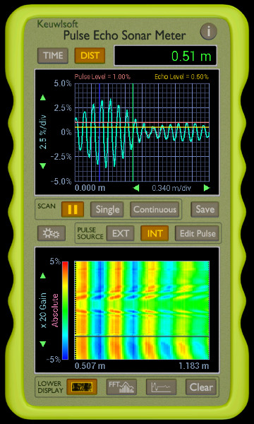
Another screenshot |
The longer guide:
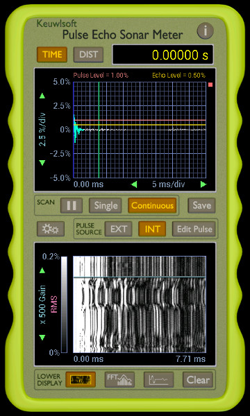
The large top display shows the recorded time-series pulse-echo signal. The trace is triggered at the pulse threshold level value and then continues collecting data for the sampling time specified in the settings (0.001 to 5 sec). The lower display can either show another time-series trace, an FFT of the data between the echo detect start and end points (blue and green lines) or an image map showing visualisation of the sound for recent scans. In settings or edit pulse mode, the bottom display will be replaced with extra control buttons.
Scan Controls
Pause – Paused state.
Single – Acquires a single scan before returning to the paused state.
Continuous – Continually acquires new scans each time the trigger level is reached.
Save
Tap on this button for the option to save a CSV (comma separated) data file with the time series and FFT data. The file will be saved in the root directory “Pulse Echo Sonar Meter Data File00000.txt” with each subsequent file being saved with a higher number. Time and date are stored in the data file. An example of file format is shown below:
Pulse Echo Sonar Meter Data File
2015-02-21 22:43:15
Time Series Data
Samples are at 44.1 kHz (i.e. one sample every 2.26757369614512E-005 s)
Sample, Amplitude (%)
1,0.5037
2,0.5230
3,0.5281
…
FFT Data
Data Points , 4096
Frequency Step (Hz) ,5.3833008
Peak Frequency (Hz) ,1162.5205304587812
Peak dB ,111.66505478253495
Frequency (Hz), Amplitude (dB)
0.0000000,38.1790
5.3833008,61.0786
10.7666016,67.4465
…
Third Octave Data
Third Octave Center Frequency (Hz), Amplitude (dB)
24.8031,
31.2500,
39.3725,
49.6063,84.38487
62.5000,87.05323
Time / Dist
These buttons determine if time or distance is shown on the x-axis of the graphs. Distance is calculated from multiplying the time by the speed of sound (340.3 m/s). The speed of sound varies with medium, elevation and pressure. Alter the sound speed in the settings mode if required. The display to the right of these buttons shows the time or distance until the echo was detected (This will be double the time/distance to the reflecting surface). An echo is detected as the time the signal first passes the echo threshold level (orange line) between the echo detect start and end limes (blue and green lines). Due to the limits of the typical microphone dB range on most devices, the echo signal might be too small to detect well unless in a location with a well defined echo. If the echo is from a nearby object, it will just merge with the pulse signal.
Pulse Source
EXT – External pulse source. The app just waits for the pulse threshold to be reached from some other sound source (e.g. clap hands to trigger).
INT – Internal pulse source. The app will generate pulses as chosen in the “edit pulse” mode. The scan will still be triggered from when the microphone input passes the pulse threshold level. Therefore in addition to the pulse output sound, other external sound sources can still trigger a scan.
Lower Display
Map - In this mode, the lower display shows visualisation of the sound between the echo detect start and end (blue and green) lines. Each scan generates one line on this image. The gain ranges from x1 to x10000 as selected by the green arrows to the left of the map. The key shows how the colour changes over the selected range. The colour can be set to depend on either the absolute or RMS value of the sound. If settings are changed, the key and gain will only apply to new data since the change occurred. Press clear to clear the map.
FFT – Generates frequency spectrum from the time series data between the echo detect start and end lines. The FFT is done with 8192 data points. If insufficient data points are available, the FFT array is zero padded up to 8192. If more than 8192 data points are present, then the time step is increased for the FFT with each data point being the average of several of the time series data points. The data is passed through a Blackman window filter prior to zero padding to reduce spectral leakage. The FFT spectrum can be displayed either as a graph, or as third octave bars. Third octave bars are based on 1 kHz being the centre of one of the third octaves. The number of third octave bins shown will depend on the amount of data selected. With little data, it is not possible to accurately determine the lower frequency third octaves. With lots of data, the time step for the FFT is increased, which also results in a reduction of the upper frequency the FFT can determine. The peak frequency of the FFT is found by fitting a quadratic around the highest point and its neighbours. The peak dB is just maximum measured dB value in the FFT. If averaging is on, the FFT graph turns yellow and the peak values are for the averaged FFT. Press clear to restart the averaging.
Trace – The %/div can range from 0.005 %/div up to 50 %/div and can be selected using the up and down green arrows to the left of the y-axis. The time per division is selected from the horizontal green arrows and can range from 0.05 ms/div up to 1000 ms/div. To pan the trace left or right in the x-axis, touch inside the graph and move in the required direction. To alter the threshold level lines or echo detect start and end lines, touch and drag them to where they are wanted. The newest trace is shown in cyan. The previous trace is in white and the one before that in grey. Press clear to clear the traces.
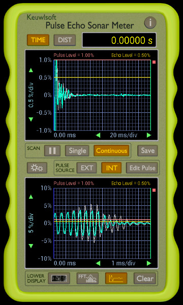
Two time trace graphs | 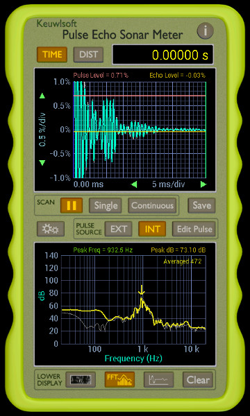
FFT graph |
Settings
Press the settings button (the one with cogs on) to replace the lower graph with some setting buttons:
Pulse Level – Set the pulse threshold level (red line) to a value between -100% and 100%. If the pulse level is positive, the scan is triggered on the signal rising past this level. If the pulse level is negative, the scan is triggered on the signal falling past this level.
Echo Level – Set the echo threshold level (orange line) to a value between -100% and 100%. The echo time is detected as the first time the signal rises past this level (positive echo threshold) or falls past this level (negative echo threshold) between the echo detect start and end (blue and green) lines.
Set Speed – Set the sound speed used for calculating distance. For example, if you have rigged up a hydrophone then you might want to use the speed of sound in water (1484 m/s). Or perhaps you live up at an elevation of 4000 m and need to reduce the speed to 325 m/s. The small display will show currently configured speed of sound.
Set Time – Set the sampling time after each triggered event. This can be set from 0.001 up to 5 seconds. The small display shows the sampling time value.
Color Map – Use a color gradient for the map images
B&W Map – Use a black & white scale for the map images
RMS – Use the root mean square values for determining the colour of each pixel in the map. Ranges from 0 to 100%.
Abs – Use the absolute values for determining the colour of each pixel in the map. Ranges from -100% to 100%.
FFT Average – Turns FFT averaging on or off.
FFT Octaves – Displays the FFT using third octave bars.
FFT Line – Displays the FFT using a line trace.
Store – Store all the current settings to one of 5 memory slots. Current settings are also saved on exiting for the next time the app is run. Use the recall button to get the defaults back.
Recall – Recall settings from one of 5 memory slots or from one of 3 default configurations.

Settings | 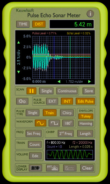
Edit Pulse |
Edit Pulse
Pressing edit pulse brings up a group of controls for configuring the internal pulse source. Note that due to hardware limitations the actual waveform may be quite different due to noise spikes as the speaker suddenly switches on/off. This doesn't normally matter, as the harsh click makes a good pulse. To reduce any harsh start to the pulse, use the envelope options to start the pulse sound more softly.
Single – Use a single waveform for the pulse source.
Train – Repeat N waveforms for the pulse, where N is the waveform count, selected from the count button.
Chirp – Sweeps the pulse output from the lower to upper of two frequencies.
Sine – Selects the pulse output to be generated from a sine wave.
Square – Selects the pulse output to be generated from a square wave.
180° - Inverts the waveform so that it goes negative first.
Freq – Set the frequency of the waveform to be generated. The frequency is shown in the small display.
2nd Freq – If chirp is selected, then a second frequency is required to sweep to. This second frequency is also shown in the small display.
Length – The length of time for the chirp pulse. This is the time to sweep from the lower to upper frequency in each pulse. Length is shown in the small display.
Count – The number of waveforms in the train mode. Count is shown in the small display.
Volume – The output volume can be set between 0% and 100%. The volume will further be adjusted by any volume buttons on your device.
Turkey - Applies a Tukey window to the waveform to soften the start and end of the pulse. The Tukey alpha is set to 0.4 such that the pulse will cosine tapper over the first and last 20% of the pulse with the central 60% being at full amplitude.
Hanning – Applies a Hanning window to the pulse.
The display, apart from showing the frequencies, chirp length and train count, also shows a graphical indication of the waveform. For a high count of waveforms in the pulse such that each wavelength fits in a couple of pixels or less, this display will not accurately show the shape of the waveform.
Finally
For Indication Only, for fun, for illustrating acoustic principles etc. Use with caution & Not for use on human subjects.
& wear ear protection if necessary as some of the pulsing sounds can become quite annoying very quickly.